自回归模型

自回归模型（Autoregression Model, AR）使用时间序列过去的数据预测其未来。$AR(p)$ 模型的形式为：$$r_t = \phi_0 + \phi_1 r_{t-1} + … + \phi_p r_{t-p} + a_t ,$$ 其中 $p$ 是非负整数，$\{a_t\}$ 是均值为 $0$ 的白噪声序列。这个模型表示，给定过去的数据时，过去的 $p$ 个值 $r_{t-1}, r_{t-2} … ,r_{t-p}$ 联合决定 $r_t$ 的条件期望。

AR模型中，$p$ 表示模型的阶数。当 $p=1$ 时，得到一阶自回归模型，即 $AR(1)$ 模型，其形式为：$$r_t = \phi_0 + \phi_1 r_{t-1} + a_t .$$

在实际应用中，AR模型的阶数 $p$ 是未知的，必须根据实际数据来决定。求解 $p$ 的的问题叫做AR模型的定阶，一般可以使用偏相关函数或者信息准测函数来决定。

在Python中生成 AR(1) 序列

根据定义，$AR(1)$ 序列的形式为：$$r_t = \phi_0 + \phi_1 r_{t-1}+ a_t,$$我们可以使用 numpy 库生成 $AR(1)$ 序列：

import numpy as np
import matplotlib.pyplot as plt

# generate data
np.random.seed(1) # 设置随机数种子
n = 1000
a = np.random.randn(n) # 生成白噪声序列

y = np.ones(n) # 初始化 `y`

# 设置参数 `phi_0` 和 `phi_1` 的值
phi_0 = 0.4
phi_1 = 0.75

# 生成 `y[i]`, 序列中的每一个数据由 AR(1) 序列的公式给出
for i in range(1, n):
    y[i] = phi_0 + phi_1 * y[i-1] + a[i]

使用 matplotlib 库画图展示序列 y ：

plt.plot(y)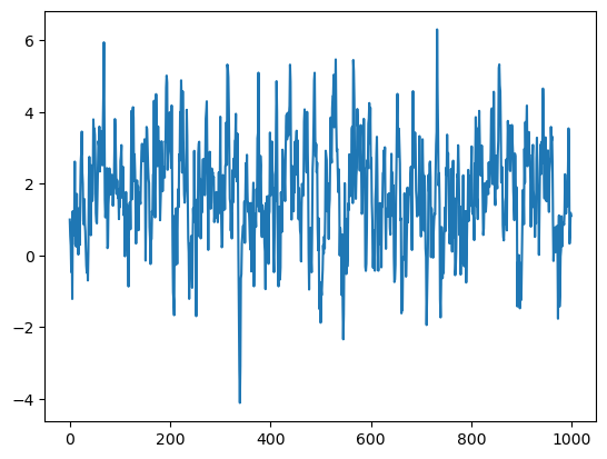

ACF和PACF

自相关系数（ACF）和偏相关系数（PACF）是两个常用的统计指标，可以通过ACF和PACF图判断待回归的序列所属的模型，以及判断模型的参数。

在Python中，可以使用 statsmodels 库中的函数方便地生成ACF和PACF图：

import statsmodels.api as sm

def draw_acf_pacf(y, lags=20):
    fig, ax = plt.subplots(2, 1, figsize=(8, 7))
    sm.graphics.tsa.plot_acf(y, lags=lags, ax=ax[0])
    sm.graphics.tsa.plot_pacf(y, lags=lags, ax=ax[1])
    # set ylim automatically
    for i in range(2):
        ylim = ax[i].get_ylim()
        ax[i].set_ylim(ylim[0], ylim[1] + 0.1)
    plt.show()

上面的代码定义了 draw_acf_pacf() 函数，对 statsmodels 库中绘制ACF和PACF图的函数做了进一步封装。下面绘制上一节中生成的序列 y 的ACF和PACF图：

draw_acf_pacf(y, lags=20)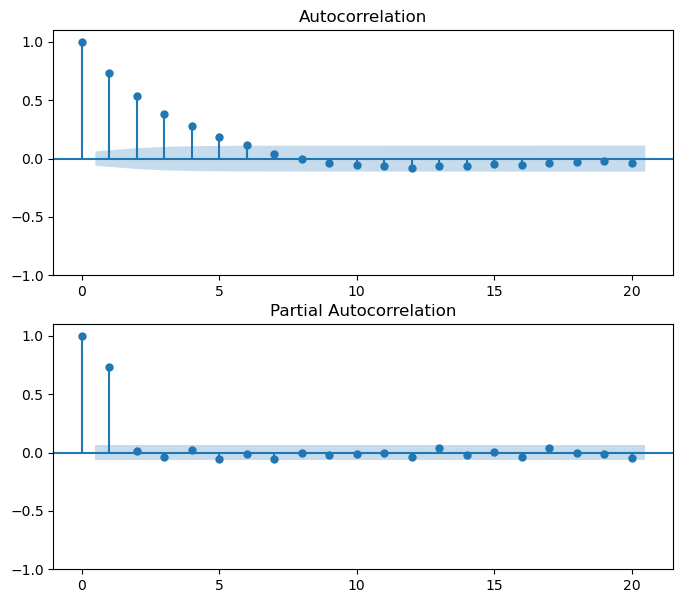

可以看出，序列 y 对应的ACF图是拖尾的，PACF图是1阶截尾的，所以可以使用 $AR(1)$ 模型拟合序列 y 。

下面使用 $AR(1)$ 模型对序列 y 进行拟合：

# 用AR(1)模型拟合数据
model = sm.tsa.AutoReg(y, lags=1).fit()
print(model.summary())

使用函数 sm.tsa.AutoReg() 调用AR模型，第一个参数为待拟合的序列，参数 lag=1 表示模型的阶数为1。

输出结果为：

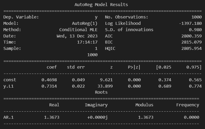
可以看出拟合结果为 $ \hat{y}_t = 0.4698 + 0.7314 y_{t-1}$，与给定的参数（phi_0 = 0.4 , phi_1 = 0.75）相比，模型拟合的效果还是不错的。

使用AR模型拟合真实数据

使用AR模型拟合标普500的滚动12个月收益率数据，数据频率为月度。首先导入数据并展示前五行：

data_url = 'https://github.com/peisong13/dataset/blob/1666949c3cb7e7908d6c9e7fb26cf1213b5d7bd6/SP500_Rolling_12_Month_Return/SP500_Rolling_12_Month_Return.csv?raw=true'
df = pd.read_csv(data_url, index_col=0, parse_dates=True)
df.head()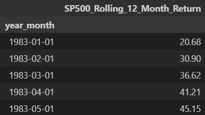

画出ACF和PACF图：

# ACF and PACF
draw_acf_pacf(df['SP500_Rolling_12_Month_Return'], lags=20)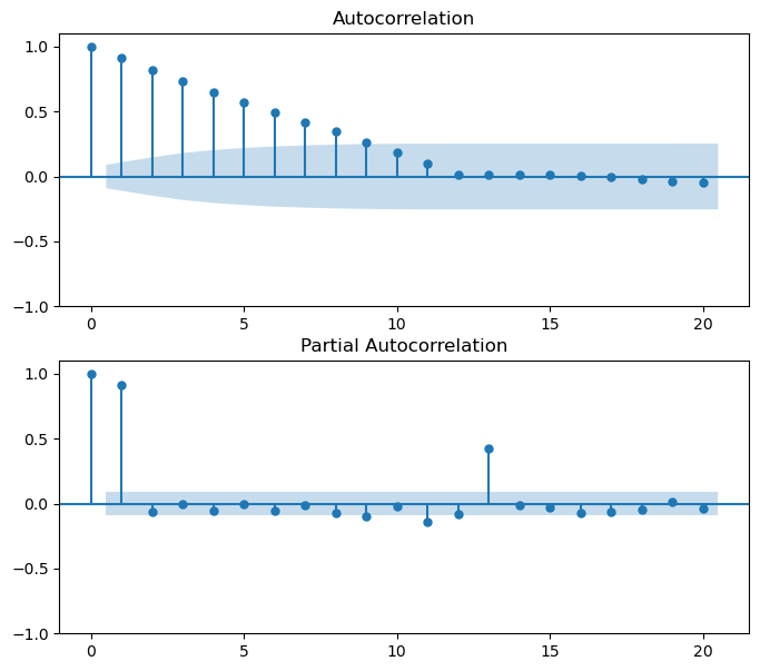

ACF拖尾，PACF 1阶截尾，因此使用 $AR(1)$ 对数据进行拟合：

# use AR(1) model
model = sm.tsa.AutoReg(df['SP500_Rolling_12_Month_Return'], lags=1).fit()
print(model.summary())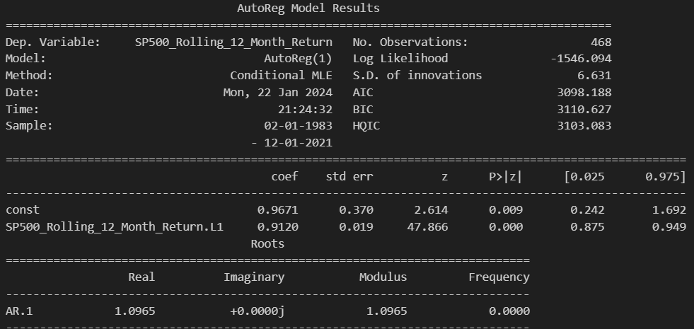

使用该模型对序列2022年1-12月的值进行预测：

# predict
pred = model.predict(start=pd.to_datetime('2022-01-01'), end=pd.to_datetime('2022-12-01'))
print(pred)

输出结果为：

2022-01-01    25.491367
2022-02-01    24.215782
2022-03-01    23.052421
2022-04-01    21.991409
2022-05-01    21.023743
2022-06-01    20.141209
2022-07-01    19.336319
2022-08-01    18.602242
2022-09-01    17.932746
2022-10-01    17.322152
2022-11-01    16.765276
2022-12-01    16.257392
Freq: MS, dtype: float64